by Scott Partridge
- Use a Motion Detector to collect distance and velocity data as a cart accelerates down an incline.
- Determine the effect of sampling rate on the time integral of velocity.
Vernier Logger Pro
ramp
Motion Detector
dynamics cart

1. Set up a ramp at a low angle (about 5 degrees), with some material at the end to cushion the impact.
2. Place the motion detector at the top of the incline.
3. Set up and configure hardware and software to collect motion data.
4. Set the sampling rate at 50 samples per second for the first trial.
5. Collect data.
6. Compare the displacement of the cart on the distance-time graph with the displacement obtained by taking the time integral of the velocity data on the velocity-time graph (the area under the curve). Record data in a table similar to the one below.
7. Repeat at the 50 samples per second rate.
8. Repeat at the following rates : 40, 30, 20, 10, 5, 3, 1.
|
Run |
|
Displacement From the d-t graph (m) |
Integral from v-t graph (m) |
|
|
|
50 |
|
|
|
|
|
|
|
|
|
|
|
|
|
|
|
Etc…
QUESTIONS
1. At what sampling rate do you obtain the smoothest distance-time and velocity-time graphs ? What factor(s) do you think affect this aspect of the graph?
2. At what sampling rate did the displacement as taken off the d-t graph match most closely the displacement as calculated from the integral from the v-t graph? This would be determined by looking at the percent difference column.
3. From what you know about integrals, how would you explain the results from #2?
TEACHER INFORMATION
ANSWERS TO QUESTIONS
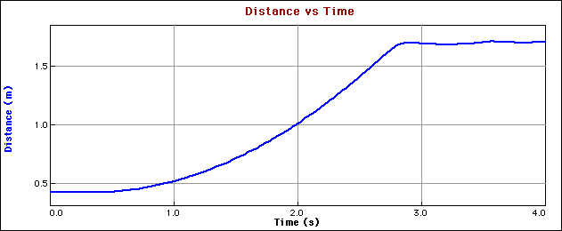
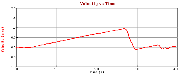
1. This lab was performed with a 3x5 card taped to the back of the dynamics cart to provide a larger area for the motion detector to reflect sound waves. As the cart accelerated, the card evidently vibrated slightly, which was only picked up at the higher sampling rates. This made the 50 sample/sec runs look "noisier"; all slower sampling rates produced graphs that looked similar to the ones below (which are from a 30 sample/sec run).If the card is not used, it is more difficult to hit the cart with the motion detector, but the graphs are all smooth curves, even at the high sampling rate.
2. In general, the higher sampling rates produced a better match between the displacement from the d-t graph and displacement from the integral off the v-t graph. From 20 to 40 samples/sec, there was no real difference in the percent difference. At 50 samples/sec, there was a slight increase, possibly due to using the 3x5 card.
3. The software program calculates the integral off the v-t graph by summing the product of the average velocity for a time interval by the time intervals. Displacement = S(v(avg) * D t). The smaller the time interval, the better the calculated displacement will be. Higher sampling rates give a smaller time interval and therefore should provide more accurate results. The results below show this to be true, except for the 50 sample per second rate, as noted in #2.
Sample results
|
|
|
From the d-t graph (m) |
Integral from v-t graph (m) |
|
|
1A |
|
|
|
|
|
|
|
|
|
|
|
|
|
|
|
|
|
|
|
|
|
|
|
|
|
|
|
|
|
|
|
|
|
|
|
|
|
|
|
|
|
|
|
|
|
|
|
|
|
|
|
|
|
|
|
|
|
|
|
|
|
|
|
|
|
|
|
|
|
|
|
|
|
|
|
|
|
|
|
|
|
|
|
|
|
|
|
|
|
|
|
|
|
|
The graphs below were collected at the 30 samples per second rate.


Back to Mr. Partridge's Home Page