---

Modified Atwood Machine

Student Report - Lab 1 of 2

Purpose:

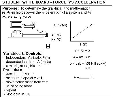
To find the mathematical and graphical relationship between force and acceleration.

Equipment:

1. Cart and track
2. Smart pulley
3. Weights, string, hanging weight holder
4. Computer interface (ULI, or equivalent)

Variables and controls:

• Independent variable = Force
• Dependent variable = Acceleration
• Controls = mass, friction, equipment set-up (if data on 2 days)

Procedure:

1. Set up equipment as shown
2. Select weights, add for total mass
3. Tilt track to compensate for friction (loaded cart rolls w/o acceleration)
4. Open ULI timer, 10 spoke pulley, set data limit to approx 20, set "trigger on gate", scale from zero, and turn on regression line
5. Accelerate system with hanger mass - take slope of V vs T curve. (if regression line fits data, the equation of the regression line gives acceleration)
6. Take mass from cart and add to hanging mass (changing force but not mass)
7. Take slope of V vs T curve
8. Record and plot Force vs Acceleration

Data:

System mass was held constant and was equal to M = 0.490 + 1.000 + 0.050 = 1.540 kg (for the cart, the added weights, and the hanging mass).

Sample of Velocity vs Time graph in Data Logger, used to get the acceleration for a point.

Data of force and acceleration copied from Graphical Analysis:

Graph of Force vs Acceleration copied from Graphical analysis

Analysis:

The graph was linear, showing a direct relation. The equation for the relationship was A = (0.631) F + .0059 However, .0059 was less than 5% of the full scale reading for acceleration (1.41 m/s²), so we consider it to be within experimental error, and set it equal to 0.

A = (0.631) F

Conclusion:

The relation between acceleration and force is a direct relationship and for our system is given by

A = (0.631) F

(Teacher information - When the students present this to the class (whiteboarding), you may want to bring out the fact that .631 is close to the reciprocal of the mass. A unit analysis can be used to strengthen this coincidence. If it doesn't come out in lab 1, you can refer back to it during the whiteboarding of lab 2.)

Modified Atwood Machine

Typical Student Report - Lab 2 of 2

Purpose:

To find the mathematical and graphical relationship between mass and acceleration, given a constant force.

Equipment:

1. Cart and track
2. Smart pulley
3. Weights, string, hanging weight holder
4. Computer interface (ULI, or equivalent)
   

Variables and controls:

• Independent variable = Mass
• Dependent variable = Acceleration
• Controls = force, friction, equipment set-up (if data on 2 days)

Procedure:

1. Set up equipment as shown
2. Select weights, add for total mass
3. Tilt track to compensate for friction (loaded cart rolls w/o acceleration)
4. Open ULI timer, 10 spoke pulley, set data limit to approx 20, set "trigger on gate", scale from zero, and turn on regression line
5. Accelerate system with hanger mass - take slope of V vs T curve. (if regression line fits data, the equation of the regression line gives acceleration)
6. Take mass from cart and remove from system (changing mass but not force)
7. Take slope of V vs T curve
8. Record and plot Mass vs Acceleration
   

Data:

The force was held constant by using a 50 g mass to produce the accelerating force of

F = 9.8 x 0.050 = 0.49 N

For this graph more data at smaller changes in mass are required to get a good graph. Data at increments of 20 to 40 grams was taken.

The graph of acceleration vs mass appeared to be an inverse, so the graph of acceleration vs the reciprocal of mass was tried.

Analysis:

The graph of M vs A appeared to be a hyperbola. A curve fit of an inverse relation was tried and seemed to work. To test this, Acceleration was plotted vs 1/Mass.


The A vs 1/M graph was linear, showing a direct relation. The equation for the relationship was A = (0.474) (1/M) + .000693 However, .000693 was less than 5% of the full scale reading for acceleration (.87 m/s/s), so we consider it to be within experimental error, and set it equal to 0.

A = (0.474) (1/M)

Conclusion:

The relation between acceleration and mass is a direct relationship and for our system is given by

A = (0.474) (1/M)

(Teacher information - When the students present this to the class (whiteboarding), you may want to bring out the fact that .474 is close to the accelerating force of .49 N. The error here is approximately 3.3%, which is within experimental error. Averaging class data gives works well here also. These labs plus a units analysis makes believers out of the students that F = MA)

The Modeling Method of teaching physics involves, in part, a series of student directed labs where students derive the laws of physics, then present their results and conclusions to the class. The introduction of dynamics is done by a standard modified Atwood machine lab. Part 1 of the lab determines the relationship between force and acceleration, with the mass held constant. The result is a direct relationship - a nice straight line graph. The students "white board" this, as shown in Figure 1. It comes out clean, and the students generally feel comfortable with the results. The fact that the slope of the F vs A line turns out to be the system mass, may or may not come out during the presentations. During whiteboarding, questions are used to help the presenters focus on key points or self-correct any errors.

Part 2 of the lab determines the relationship between the system mass and the acceleration, with the force (hanging mass) held constant. The results give an inverse relation, which the students linearize to get the equation. A whiteboard of this lab will involve identifying that the slope of the line is the inverse of the force. If the students didn't discover the point in the first lab that the slope was close to the inverse of mass, that point is rechecked by the students. The combination of the labs nails down the equation for Newton's second law from both directions.