
 |
Factors are equal for both variables |
 |
Graph is a straight line |
 |
Ratio of Dependent/Control is a constant value |
For a direct relationship, when we double the value of the control variable, the dependent variable doubles, also. When the control is tripled, the dependent also is tripled. If we reduce the size of the control to a third, the dependent is also reduced to a third. |
|
 |
Factors are reciprocals for the variables in each column |
 |
Graph is a downward curve |
 |
Taking the reciprocal of the control, you get a straight line graph |
 |
Ratio of Dependent/(1/Control) is a constant value |
For an inverse relationship, when we double the value of the control variable, the dependent variable is reduced to half its former value. When the control is tripled, the dependent is reduce to a third. If we reduce the size of the control to a fourth, the dependent becomes four times larger. Hence the "inverse" nature. |
|
 |
Factors of the dependent variable are squares of the factors for the control variables |
 |
Graph is an upward curve |
 |
Taking the square of the control, you get a straight line graph |
 |
Ratio of Dependent/(Control2) is a constant value |
For a square relationship, when we double the value of the control variable, the dependent variable becomes four times larger. When the control is tripled, the dependent becomes nine times larger. If we reduce the size of the control to a fourth, the dependent becomes 1/16 as large. The dependent variable grows and contracts faster than the control. |
|
 |
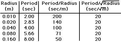
Factors of the dependent variable are square roots of the factors for the control variables |
 |
Graph is a curve which gets less and less steep as it goes to the right |
 |
Taking the square root of the control, you get a straight line graph |
 |
Ratio of Dependent/(Control2) is a constant value |
For a square root relationship, when we double the value of the control variable, the dependent variable becomes only the square root of two times larger. When the control is quadrupled, the dependent becomes two times larger. If we reduce the size of the control to a fourth, the dependent becomes 1/2 as large. The dependent variable grows and contracts slower than the control. |
|
This summary applies only to the four relationships we studied and the four techniques of looking at them we used. There certainly are other mathematical patterns which will be uncovered as we study physics throughout this school year.
EXTENSIONS All of the relationships we study during this set of web pages are what is known as Power Relationships. In a power relationship, the dependent variable is proportional to the control variable taken to some power. For example, the four relationships we had could be written as below, including the equation form:
Direct y a x1 y = k x1 Inverse y a x-1 y = k x-1 Square y a x2 y = k x2 Square Root y a x0.5 y = k x0.5 General Power y a xn y = k xn If we employ a graphing calculator that can do regression analysis, or if we use a computer graphing program that can do curve fitting, we could simply ask it to do a power regression or power fit. If the result indicated is one of these powers, we would know what to call it. Examples of programs we may use are Excel and Graphical Analysis.
Often, though, with real data, the result may come out something like 0.96 or 1.05. For the level of our work, this is indicative of a direct relationship in either case. We have to be prepared for "close" rather than exact results.
On the other hand, if the power is close to 3, we might conclude that the relationship is a cubic one. The dependent variable depends on the control variable raised to the third power.
Log-Log Plot
One additional way of analyzing power relationships is to plot the logarithms of both the control and the dependent variables. If the relationship is a power, the graph is a straight line with a slope equal to the power.
The theory on this is shown here:
y = xn Take the natural log (ln) of both sides:
ln y = n ln x
ln y / ln x = n = slope of graph = power
Updated August 2001